Speech Bubbles
This short video shows how to use the speech bubbles report functionality for the Forensic Browser for SQLite. This new report option will be available in version 3.3.0 which will be released shortly.
This short video shows how to use the speech bubbles report functionality for the Forensic Browser for SQLite. This new report option will be available in version 3.3.0 which will be released shortly.
Often data held within tables in databases is stored within a BLOB (Binary Large OBject) this data is often structured data that is encoded in a particular format. XML and Binary Plists are examples of these structured storage objects. Often the data in each blob in a table is in the same format and it would be useful to query these objects and include selected data in a report.
The Structured Storage Manager does this by using a template to break down the items in each BLOB object and converts the data to a table held within the case file.
The following screenshot shows the msg_blob records from the messages table in a Facebook orca2.db file. The blobs are shown in their raw (hex) form and are clearly a binary (non-text format) and thus it is not possible to query these objects using normal SQL commands:

We can decode the data by :
Create a case file and then open the Facebook orca2.db (the decoded data from the orca blobs will be written to a new table in the case file).
Then invoke the structured storage manager from the Tools menu:

In the following dialog we need to provide some data:

Source table (main.messages) is the database.tablename that contains the blob column
ID field (msg_id) is the primary key of this table – we need something unique so that a query can be made tying the extracted data back to its source
Structured Storage field (msg_blob) is the field/column that contains the blob data
Destination table name (StructuredStorage_messages) i steh name of a new table that will be created in the case file that will hold the extracted data
Strcutured storage type (Facebook orca blob) is the encoding type used to store the structured data selected from the list of currently supported types
Once all the above has been selected we are ready to decide which items from the decoded blob we want to select to copy to the extracted data table. The simplest solution here is to select “Add all elements” from the pop-up menu:

The Browser will then parse a structured storage blob and decode each of the data types and create tree structure that represents the underlying datat and create an associated table with a new column for each element.
The following screenshot shows the decode orca blob structure:

You can select a subset of the above but as all of the data is added to individual columns in a new table it is easier to use the SQL features of the Browser to select your chosen columns.
The screenshot below shows a JOIN created on the two tables and just those I require (containing the msg_id, date, userID, message text and senderID) are selected for my custom report:


I recently saw a Twitter conversation where a user wanted to see the EXIF data from some image files displayed as maps and showing a clickable URL for Google Maps. The latter part of this problem can easily be solved with the Browser – the steps are as follows:
This example assumes that you want to display the locations of all the files in the path “E:\\My Pictures”
1. Run exiftool and export the relevant results as a csv
Run the following command line in exiftool
Code:
exiftool -n -gpsposition -csv "e:\\my Pictures" > "e:\\geo.csv"The commands instruct exiftool to parse all of the data in the specified folder and pipe the output in csv format to the specified file.
-gpsposition specifies that just the GPS tags from the EXIF data will be exported
-n tells exiftool to save GPS data in numerical (floating point) form
A few of the lines from the exported geo.csv file are shown below:
Code:
e:/my pictures/hugh.jpg,

e:/my pictures/image.png,

e:/my pictures/image1.JPG,50.0867083333333 -5.31498611111111

e:/my pictures/IMG_1568.JPG,50.0888333333333 -5.10166666666667

e:/my pictures/IMG_1697.MOV,50.1567 -5.0683
We can see that for those files that have GPS information it is displayed as a lat and long. The keen-eyed among you will have noted that the lat and long is actually a single column, i.e. there is no comma separating the two – this can be resolved later with the Forensic Browser.
2. Import the csv into an SQLite database
Using the sqlite command line tool (or another tool of your choice) create a new database:
Code:
sqlite3 geo.dbNow within the command line tool create a table with two columns for the new data
Code:
CREATE TABLE files (filename TEXT, latlon TEXT);Set SQLite to work in csv mode
Code:
.MODE CSVimport the csv file created with exif tool.
Code:
.IMPORT geo.csv3. Use the Browser to create a query and then a VIEW displaying the lat and long as two fields
A query showing the data from the files table looks as follows:

What we need is a query that splits the lat and long from the latlon column into two separate entities, i.e. two new columns. SQLite provides an inbuilt function to extract a portion of a field SubStr and a second function InStr to find the offset of a particular element of a string.
Notice that in the latlon field above the two elements are separated by a space, the following query extracts the characters from the latlon field starting at character 1 and stopping at the character 1 before the space.
SubStr(files.latlon, 1, instr(files.latlon, ‘ ‘) – 1)
This can be combined with a similar query that extracts the part of the latlon string after the space. The combined query looks as follows:

4. Create a VIEW to represent this query
A VIEW is a sort of virtual table and the VIEW can then be used in place of the query itself. The SQLite command we would use is:
Code:
CREATE VIEW geo AS (SELECT files.filename,

  files.latlon,

  SubStr(files.latlon, 1, instr(files.latlon, ' ') - 1) AS lat,

  SubStr(files.latlon, instr(files.latlon, ' ') + 1) AS lon

FROM files)

5. Use the Browser to display a map for each row showing the location defined by the lat and longs
The Browser has a built-in function that creates geolocated maps based on lat and long fields:

You are just prompted for the table, an ID field and the lat and long columns:

A new table is created and populated with maps for each row in the “source” table. Once the maps have been created for you a simple visual query is automatically built joining the two tables allowing you to customize your query:

6. Use the Browser to combine the lat and longs into a clickable URL
The final step is to create a URL column. This simply uses some hard-coded string values concatenated together with data from the lat and lon columns we created above.
The format for a google maps URL at zoom level 9 is as follows:
http://maps.google.com/ll=
All we need to do is replace the
The SQL for this row is below:
‘http://maps.google.com/?ll=’ || CaseDB.Geodata1.lat || ‘,’ || CaseDB.Geodata1.lon || ‘,z9 ‘ AS url
Hardcoded strings are enclosed in single quotes and the SQLite concatenation operator || is used to join successive strings and field values together, we call the column URL.
The final report is shown below

A. When a journal is in use (potentially).
The raison d’etre for a journal, be it a traditional rollback journal or the newer SQLite Write Ahead Log (WAL) file is to maintain database integrity. Simply put if an operation fails for whatever reason then the changes to the database are unwound to put the DB back to its last known good state. It might seem obvious then to state that a copy of securely deleted data would need to be kept in order to facilitate this functionality. This securely deleted data can and sometimes does exist for quite some time.
We also need to understand that SQLite groups actions together in transactions, transactions can be one database update (write, modify, delete) or it can be many thousands of such actions as determined by the user. Think of a simple messaging application whereby a message is received asking to be “friends” – our hypothetical app needs to write the friend request to the messages table and add a user to the users table. It would make no sense to update the messages table with a message that referred to user x when user x’s details had not yet been added to the users table, so both these actions could be wrapped in a transaction so either both tables are updated or neither is updated.
So how does this impact secure delete?
First we need to understand what secure delete does, according to the SQLite website the command (pragma) that initiates secure delete says “When secure-delete is (sic) on, SQLite overwrites deleted content with zeros.”
Well that gives me a warm fuzzy feeling, when I delete it, it’s gone! But hang on, if SQLite immediately overwrites something I delete and something goes wrong before the transaction completes how can SQLite rewind the DB to its last good state?
The simple answer is it can’t. in order to maintain database integrity SQLite MUST maintain a copy of the data that has been deleted somewhere until it ‘knows’ the last transaction has completed correctly, that somewhere is the journal.
Rollback Journals
Lets look at an example with a rollback journal. For the purposes of this demo I do the following:
Also unless you specifically tell SQLite differently it treats each individual database update as a transaction, so I group the updates into sets of 4 so each of the 4 updates forms a transaction. The simplified instructions I use are as follows:
Code:
begin transaction;
insert into users (1, 'System');
insert into users (2, 'Helen');
insert into messages (1, strfTime('%s','2016-03-01 09:12:45'), 0, 1, 1, 'Hello welcome to Sanderson Forensics test messaging database');
insert into messages (2, strfTime('%s','2016-03-02 15:08:14'), 1, 1, 2, 'Hi Honey just got this new messaging app - it''s awful :)');
end transaction;
begin transaction;
insert into messages (3, strfTime('%s','2016-03-02 15:10:12'), 0, 1, 2, 'Sounds great - another app, I''m soo excited');
insert into messages (4, strfTime('%s','2016-03-02 15:12:45'), 1, 1, 2, 'haha, thought you''d like it');
insert into messages (5, strfTime('%s','2016-03-02 15:14:42'), 1, 1, 2, 'anyway i''ll be home in a couple of hours hour xx');
insert into messages (6, strfTime('%s','2016-03-03 17:12:45'), 1, 1, 2, 'just left the office....');
end transaction;
begin transaction;
insert into messages (7, strfTime('%s','2016-03-04 09:02:01'), 1, 1, 2, 'just got to work');
insert into messages (8, strfTime('%s','2016-03-04 09:10:12'), 0, 1, 2, 'cool have a nice day x');
insert into messages (9, strfTime('%s','2016-03-04 09:22:02'), 0, 2, 1, 'Paul, be my friend, Darcy');
insert into users (3, 'Darcy');
end transaction;
begin transaction;
delete from messages where id < 4;
insert into messages (10, strfTime('%s','2016-03-04 09:25:43'), 1, 1, 3, 'Hiya mate - didn''t know you were on this app');
insert into messages (11, strfTime('%s','2016-03-04 09:27:43'), 0, 1, 3, 'No time for pleasantries, Ive transferred the money from the company account');
insert into messages (12, strfTime('%s','2016-03-04 09:29:22'), 0, 1, 3, 'This is really scary - I dont do illegal - no more after this');
insert into messages (13, strfTime('%s','2016-03-04 09:29:22'), 1, 1, 3, 'OK good - thats it we are quits now');
end transaction;
begin transaction;
insert into messages (14, strfTime('%s','2016-03-04 10:03:21'), 0, 1, 2, 'Hi honey - are you working late? what time will you be home?');
insert into messages (15, strfTime('%s','2016-03-04 10:05:10'), 1, 1, 2, 'about 8pm hopefully');
insert into messages (16, strfTime('%s','2016-03-04 13:13:40'), 0, 1, 3, 'Oh - I forgot to say, delete any trace of this conversation');
insert into messages (17, strfTime('%s','2016-03-04 14:08:21'), 0, 1, 2, 'Hi honey - did you get my message form earlier?');
end transaction;
insert into messages  (18, strfTime('%s','2016-03-04 17:05:08'), 1, 1, 2, 'been in a meeting, leaving shortly, quick pint with the boys and then ill be on the train');
delete from messages where id = 11 or id = 12;
end transaction;
Before we look at the recovered data with the Forensic Browser for SQLite a quick summary of how a rollback journal works.
Essentially before a change to a page in the database is made the page is copied to the rollback journal. The database is then updated and only when this is successful the rollback journal is invalidated by wiping the journal header (in fact the default mode is to delete the rollback journal file in its entirety - more on this later). If something goes wrong e.g. the application/devices crashes. When it is restarted the valid rollback journal is still there so SQLite will know there has been a problem and will transfer the cached/saved records back into the database to restore it to its last known good state.
When opening a database with the Forensic Browser for SQLite if there is an associated journal or WAL then the user is prompted as to whether they want to process this also. All records from both the database and the journal/WAL are then added to the parsed data and marked as to their source:

The following screenshot shows an SQLite database and its associated journal loaded into the Forensic Browser for SQLite. You can see that the records that are in the DB are marked as live and that records 1-3 and 11 & 12 are missing as we expect.

The journal however still has a copy of the deleted records 11 & 12, from the last transaction. Records 1-3 have been overwritten in the journal by the subsequent transactions since they were deleted.
So while the journal exists the secure delete is not as effective as you may think. To be clear this is an intended consequence of the operation of SQLite and should not be considered a bug.
It is also useful to consider when we may find helpful data in a journal. Rollback Journals held on disk operate in one of three modes, delete, truncate and persist. These three modes work as follows.
When a journal is in delete mode (the default) and a transaction is completed successfully the journal file is deleted. In this instance, the journal could potentially be recovered using normal forensic techniques and any securely deleted data from the last transaction recovered.
When a journal is in truncate mode and a transaction completes successfully, the journal file size is reset to 0 bytes, the file is truncated. As above the content of the truncated journal could potentially be recovered forensically and securely deleted records from the last transaction recovered.
When a journal is in persist mode (this is the mode I used for my demo) and a transaction completes successfully, the header for the journal file is overwritten but otherwise the journal stays on disk and of course, all securely deleted data from the last transaction will be easily accessible.
WAL Journals
What happens when we do the same operation with WAL files? This is much more fun
First - how do WALs operate? The explanation for the SQLite web site is that they turn traditional journaling on its head and that rather than copying the page that will be changed to the journal they leave the original page in the database and write the new page to the WAL.
The database reader when it needs to read a page looks for the latest copy in the WAL and only reads the main database if it can't find a copy in the WAL.
The database is always left in a good state as any errors (power cuts etc.) will only affect writes to the WAL.
There is another difference/complication. Rather than copy the changed pages from the WAL to the database after every transaction, multiple transactions are appended in the WAL one after another until a WAL 'checkpoint' occurs. By default, this is when a transaction takes the WAL above 1000 pages of data, if the application specifically triggers one or when/if the application shuts down gracefully.
At a checkpoint, all changes pages are written back to the main database file. However, after a successful checkpoint, the WAL is not deleted or truncated, any new pages start to be written from the start of the WAL file leaving all older pages in a sort of WAL slack.
The WAL file is only deleted when the application is shut down gracefully and all of the changed pages in the WAL have been successfully written to the database.
After opening the database and associated WAL in the Forensic Browser for SQLite the summary of the data in the messages table is as follows. As you can see from the messages marked as true in the sfIsLive column the live records are missing records 1, 2, 3, 11 & 12 as we expect:

We can also see multiple copies of the securely deleted records 1-3 and a copy of the securely deleted records 11 & 12.
There are multiple copies of records 1-3 which were in database page 3 because each time page 3 was updated a new copy of it was written to the WAL. We can see that records 1-9 where all in DB page 3 at some time and also see that page 3 was updated in commits 1, 2 & 3.
Of interest, we can get an idea of what SQLite is doing in the background as we can see that message ID 4 has been in both DB page 3 and DB page 4 and so at some point, SQLite has moved these records within the DB.
We can also see that there are no pages of data actually in the database, this is because in our example a checkpoint has not yet occurred and all pages are waiting to be written to the main database file.
As stated writes to WAL files start at the beginning of a file after a checkpoint takes place. WAL files are deleted when the application shuts down (after any associated successful checkpoint). So if a WAL file exists or can be recovered then it may be possible to recover records from multiple previous transactions.
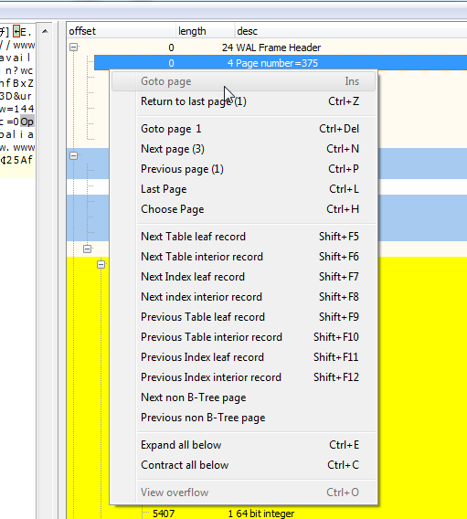
There is a further feature in the Forensic Browser for SQLite that allows you to "look" at a database as it used to be. When you open a DB and choose to process the associated WAL the Browser will ask "which is the last commit frame that you want to use?". Typically this will be the latest but by choosing an older commit frame you can get the Browser to show you the database as it was when that frame was the last to be written. Essentially you can wind back the clock on the database state.

The table below shows the database when commit frame 5 was the last live frame. In the screenshot, you can see that records 1-3 have yet to be deleted and that records 7 onwards have not yet been written (although they are still shown as this is a forensic tool after all).
So in summary:
If a journal file exists or can be recovered then you can potentially find evidence of any securely deleted records from the last transaction.
If a WAL file still exists or can be recovered you can potentially find evidence of any securely deleted records from often many previous transactions.
The Forensic Browser for SQLite incorporates features such that you can right click on a numeric date column and have the Browser convert a number to one of the supported date formats, applying a timezone offset as required.
The process is simply – right-click the required column and choose “View column as…”.

Select the date format that you believe the column is saved as, in this case I recognise this as an IOS NSDate format:

And it’s that simple…

So how can we validate the conversion done by the Forensic Browser? The method I choose is to use the SQLite built in functions within the Forensic Browser, as follows.
We can do this by simply having two copies of the column that we are converting within the same query an dthe using the SQLite DateTime fucntion to convert and display the date, the SQL is as follows:
SELECT ZKIKMESSAGE.ZTIMESTAMP,
DateTime(ZKIKMESSAGE.ZTIMESTAMP + 978307200, ‘unixepoch’) AS SQLiteConvertedTime,
ZKIKMESSAGE.ZBODY
FROM ZKIKMESSAGE
* The first line selects the ZTIMESTAMP column (and we apply an NSDate conversion using the Browsers built in features as above)
* The second line selects the ZTIMESTAMP column again, does some internal SQLite stuff – more shortly) and displyas it in a column with the alias SQLiteConvertedTime
* the third column adds the ZBODY field just so we can reference teach row to the screen shot above
* and finally the fourth row specifies the table we are using
The results of this query are as below:

As you can see the timestamps are the same and the two date columns compare as expected. The beauty of this method is that you do not need to leave the Browser but you are directly calling a function (DateTime) from the SQLite3.dll and thus bypassing the Browser for an independant date validation.
So how does it work?
The Browser takes the numeric value from the ZTIMESTAMP column adds 978307200 to it and then tells SQLite to convert it to a human-readable string and treating the new number as a unixepoch date.
DateTime(ZKIKMESSAGE.ZTIMESTAMP + 978307200, ‘unixepoch’)
The NSDate format records the number of seconds since 1/1/2001 and the unix date format records the number of seconds since 1/1/1970. 978307200 is the number of seconds between the two dates (often referred to as the Delta), this figure is added to adjust the NSDate value to a unix value.
The relevant web page for the DateTime function is as follows:
https://www.sqlite.org/lang_datefunc.html
Unix 10 digit dates
The number of seconds since 01/01/1970
Unix dates can be validated simply by using the date “as is”, i.e. there is no need to apply a delta
The SQL query is:
DateTime(numeric_time, ‘unixepoch’) AS Converted,
Unix milliseconds (13 digit) dates
The number of milliseconds since 01/01/1970
as above but convert to seconds by dividing by 1,000
The SQL query is:
DateTime((numeric_time / 1000, ‘unixepoch’) AS Converted,
Unix nano second and 100 nano second dates
These are the same as above but use 1,000,000,000 and 10,000,000 respectively as the divisor.
Chrome/webkit time
This is the number of microsecond intervals since 01/01/1601
The Delta (difference) between 01/01/1601 and 01/01/1970 is 11644473600 seconds, so first convert the Chrome date from microseconds to seconds by dividing by 1,000,000 then just take away the delta (we take it away because the chrome epoch date [01/01/1601] is older than the unix epoch)
The SQL query is:
DateTime((numeric_time / 1000000) – 11644473600, ‘unixepoch’) AS Converted
Windows 64 bit filetime
This is very similar to the Chrome date except the interval is the number of 100 nanoseconds since 01/01/1601. Therefore instead of dividing by 1,000,000, we need to divide by 10,000,000
The SQL query is:
DateTime((numeric_time / 10000000) – 11644473600, ‘unixepoch’) AS Converted
NSDate (IOS)
Records the number of seconds since 01/01/2001
The SQL query is:
DateTime(numeric_time + 978307200, ‘unixepoch’) AS Converted
Mac
Records the number of seconds since 01/01/1904
The SQL query is:
DateTime(numeric_time – 2082844800, ‘unixepoch’) AS Converted
OLE Automation
Records the number of days and fractions of a day since 30/12/1899
Using an “example date” of 42439.766146 the query we want is:
SELECT DateTime(42439.766146 * 86400 – 2209161600, ‘unixepoch’) AS Converted
i.e. convert the fractional day portion into seconds by multiplying by the seconds in a day.
Creating a custom report on the Kik messenger database
In this article, I want to take you through the process of creating a custom, but simple, report on a Kik messenger database step by step. As we work through the process we will choose which columns we think will be useful in our report and modify our report by creating simple visual SQL joins on different tables.
The first step when looking at a new database is to have a quick look at all of the tables to get a feel for the data that’s in them and see how we might start building our report. I use the “summary tables” tab to quickly review each table, in turn, there are three tables that seemed to immediate deserve some further attention:
XKIKMESSAGE – Contains the message text and some timestamps but does not contain a user name, it does, however, have a ZUSER column which would seem to be a user number.

There is also a ZKIKUSER table with user details, this almost certainly links to the ZKIKMESSAGE table and Z_PK (Primary Key) is almost certainly the user number referred to above.

Finally there is a ZKIKATTACHMENT table again with a timestamp column and a content column that could do with some further investigation

The first query is a visual query linking the ZKIKMESSAGE table with the ZKIKUSER table so that we can attribute a user name to each message. I won’t go into the mechanics of all the different types of JOINS available in SQLite here (there is an article dealing with this on my web site), I will just say that as we want a join with every row in the messages table matching up with a row from the users table, we need a LEFT JOIN (the Forensic Browser default). I’ll also now start to select the different columns that I may want in my final report (I can always change this later). In the animated gif below you can see the process and watch the SQL commands being built for you:
Because I like to start to tidy my reports up early I can now choose to display the two dates in a more meaningful format. In this table in Kik the dates are Mac Absolute format so I choose that format for all values in a column by right clicking on the relevant column and selecting the “display as” menu option. I can then choose the display format and timezone (I’ll set this to Mountain Standard Time).

So what about attachments? The first thing to do is to JOIN the attachments table in the same way as we did the users table. From the summary tables above we can see that the best join candidate is to use the Z_PK (primary key) of the messages table and the ZMESSAGE field of the attachment table. We will again use a LEFT JOIN as we want all the rows from the messages table and just the matching values from the ZKIKATTACHMENT table (where there is no match any new columns will be blank). I have chosen to include the attachment timestamp and the content columns form this table. Again we can see the SQL commands being built and starting to look quite complex although we have not typed a single line of SQL code.

This report gives us a column with a date for any attachment and a column called “content”. Further research shows that strings in the content filed are file names and that these files are binary Plists that contain jpgs (the attachments). How these Plists are decoded is beyond the scope of this article (there is another on my web site that deals with these), however, there is a Forensic Browser extension callable from the extensions menu that decodes these Plists and imports the jpgs within each Plist into a new table within the Browser case file. It is then a simple matter to make a final JOIN on this new table to include these pictures in the report. I finally add “is not null” to the column holding the picture to display just those messages that related to an attachment.
The animated gif below shows this process: the extension is run, a JOIN is made on the new table, a report is executed and then modified to show only those records that refer to attachments.

It is worth noting here that most forensic software that creates a nice ‘canned’ report on an application only displays those tables and columns that the developer deems important. For instance, the Skype contacts table at the last count contained 97 columns and the messages table has 36 columns. While these reports usually contain all of the relevant data there can often be additional very useful and relevant data held in columns that do not form part of the generic report.
Additionally, database developers are prone to changing the schema of a database without notifying anyone; this may break your forensic application or may introduce relevant data in a new column. Database schemas also often vary between platforms, with a different schema for, say, Kik on Android than on IOS and different schemas might mean the best report on one platform differs from another.
The areas I will cover, with examples and screenshots, are:
Many SQLite applications allow the user to delete records as part of their operation and databases by their nature are often dynamic with new records being added and pages of B-Trees being moved to maintain a valid B-Tree structure. Pages (possibly containing live and deleted records) are often copied to rollback journals or in the case of the newer Write Ahead Logging journal, the new pages are written to the journal and the old page containing redundant data is left in the database.
All this means that if records have been deleted and/or a journal is present then the deleted records need to be found and the journal processed so that we can see and report on both the live and any deleted data.
Extraction of records that may have been deleted and partial records (see the article on my website that covers this in more detail) is straight forward with the Forensic Browser, as is processing any associated journals (both the old rollback journal and the newer WAL journal). You just need to choose your source database and when prompted select the options that you want.

Creating a query to show the content of the table can be done by just dragging a table to the visual query designer window and check to mark which fields you want in your report. The SQL is generated automatically for you. Drag the mouse between columns in different tables to create simple or complex joins – all visually:


After selecting just the records we want, from the source we want a common requirement is to restrict the report to one that contains messages from specified users and just within a given timeframe.
Again this is straight forward and in the same manner, as we selected the records from the journal we can add a further filter on the from_dispname column and just choose selected users from the Skype database:


Many databases maintain pictures such as avatar pictures (Skype) and message attachments (WhatsApp) some forensic applications will display these pictures alongside the appropriate data but most SQLite browsers are not designed for this. Many applications however store pictures outside of the database, Blackberry messenger stores attachments as individual jpgs in the devices file system, some versions of Kik messenger store the attachments embedded within individual binary plists stored on the devices file system.
Irrespective of the method used the Forensic Browser is able to display these pictures alongside the message to which they relate. Displaying a blob as an image is trivial in the Forensic Browser, either choose to display all blobs as pictures or right click on a column and choose to display just that column as a picture:


For more complex import scenarios such as Kik messenger where the pictures are stored external to the database in binary plists, Browser extensions can be written to perform the import task. See the article re Kik messenger pictures on my web site.
This article describes how WAL files work and how to deal with them forensically – the steps are very straight forward with the Forensic Toolkit for SQLite and the article takes you through them. I will go into a little detail regarding the format and usage of a WAL file, some of the forensic implications of recovering data and present two methods for recovering the data without missing or overwriting existing records.
In order to maintain database integrity, SQLite often makes use of WAL files. At a very basic level, WAL files are easy enough to incorporate into a parent SQLite database – you just need to open the parent database in SQLite. WAL files are a form of cache whereby data that is written to an SQLite db is first written to the WAL file (when this is enabled) and then at a later time (known as a checkpoint) the SQLite data is written into the main database. So from a forensic viewpoint, the existing database is an older version of the data and when the WAL is checkpointed you see the current version.
So to incorporate a WAL file just open the main db in SQLite. SQLite will see the existing WAL file in the same folder as the main database and will assume that an error has occurred (application/computer crash) and will automatically checkpoint the WAL file and add the changes to the main database.
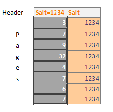
SQLite writes a value known as a Salt to the WAL file header, this salt is also written to each frame header for each page in the WAL file (the page header and page data itself are known as a frame).
So if pages 3, 7, 9, 32, 4 are updated (in that order) and the salt is 1234 then the WAL file will look as follows.

So in the same checkpoint if pages 7, 6, 7 are updated (in that order) the salt is still 1234 then the WAL file will look like this:
A checkpoint occurs when the WAL files reach 1000 pages (this is configurable in SQLite) or when the programmer forces one. At this point, each page will be written back to the main database in order so only the last version of page 7 in our example would be seen by an investigator using SQLite to write a WAL file.
It gets more interesting though. When a checkpoint occurs then the WAL file is not deleted, rather the next set of pages are written from the start of the WAL file.
SQLite determines what is current by means of the salt value and to do this it ensures that the salt value changes for each checkpoint.
Our example below shows our WAL file after a checkpoint has occurred and then three new pages have been updated – pages 5, 7 and 2. This new WAL file has the new salt (6789) written to the header and to each new frame header. So when SQLite writes the content of a WAL file back to the database, it first reads the salt from the WAL header and checks each frame in the WAL file to make sure that the salt matches – when it reaches a salt that doesn’t match it stops writing data. This means that any frame in the WAL file that has a different salt will never be written back to the main database (essentially this has already happened at a previous checkpoint). This data could of course be forensically valuable.
It can be seen from the image below that the WAL file contains 5 pages from the previous checkpoint, without tools such as SQLite Forensic Explorer there is no way to look at the contents of these pages in “WAL Unused”.

So how can we examine a WAL file?
Forensically the normal method of looking a at WAL file is to take advantage of the fact that when an SQLite database is opened if a WAL file is present then the content of the WAL file will be written to the main databases (i.e. it is checkpointed). There are a number of problems with this approach.
1. Old data in the main database file is overwritten by the data from the WAL file potentially losing evidentially valuable data
2. The WAL file may contain more than one version of a page
3. The WAL file could contain deleted data in unused space
4. WAL files can contain data that has previously been written (checkpointed) to a database and may subsequently have been overwritten
It follows therefore that a better approach could reveal evidence that might otherwise be lost – There are two methods:
1. Use Forensic Recovery for SQLite to carve all the records from the WAL file and insert them into a new database
2. Use SQLite Forensic Explorer to look at the WAL file page by page.
I will discuss both methods:
SQLite Forensic Recovery and Explorer are only available as part of the SQLite Forensic Toolkit, more information here.
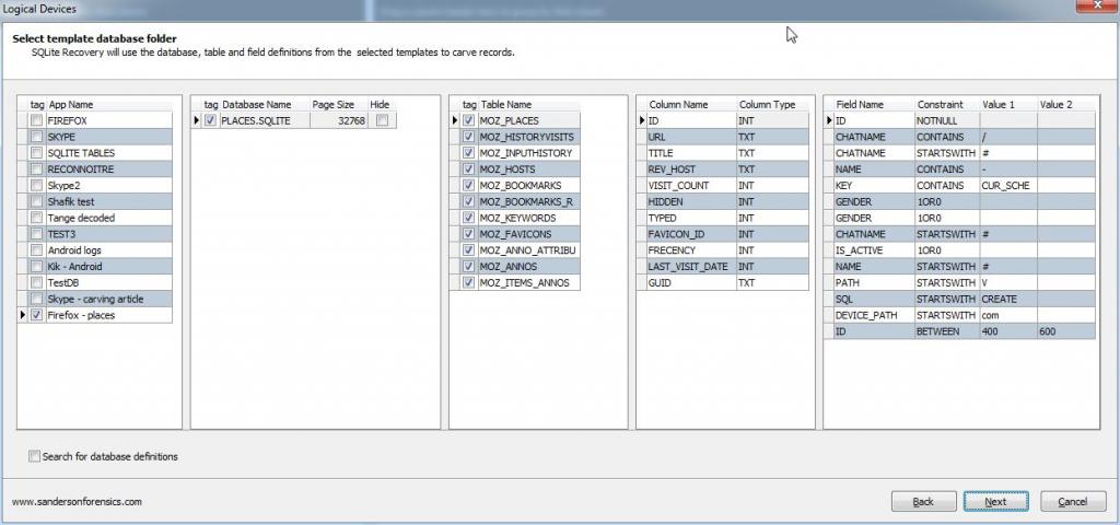
This solution is the simplest one, Use Forensic Recovery for SQLite to carve directly from the WAL and create a new database with just the records from the WAL. All we need to do is ensure that a template is created for the Database, this can be done by just pointing Forensic Recovery for SQLite at the existing database (the DB associated with the WAL) when following the wizard. Forensic Recovery for SQLite will display tables as per the original schema (with constraints removed so duplicate records are allowed) showing all of the records, it also creates a new SQLite database that we can examine with the Forensic Browser for SQLite. The steps are:
Finally select the output folder for the carved database and hit “Finish”

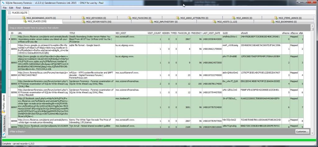
Once the carve process has completed, a few seconds, you can view each table in turn and review the carved records. Note that the recovered records in this table are logged as “mapped” rather than “Live” as they are not currently live in the associated database (the WAL has not be written to)
Double-clicking on any entry above will take you to a table showing exactly where (byte offset) in the WAL file the recovered record was located.

While SQLite Forensic Explorer can read and decode pages and records in pages from a WAL file individually, a better solution is obtained if the table schemas from the database that is associated with the WAL file are available to SQLite Forensic Explorer. When this additional information is available the records from WAL file pages can be correctly decoded and presented to the examiner in easier to read grid form.
The process of investigating an SQLite WAL files with SQLite Forensic Explorer is simple.
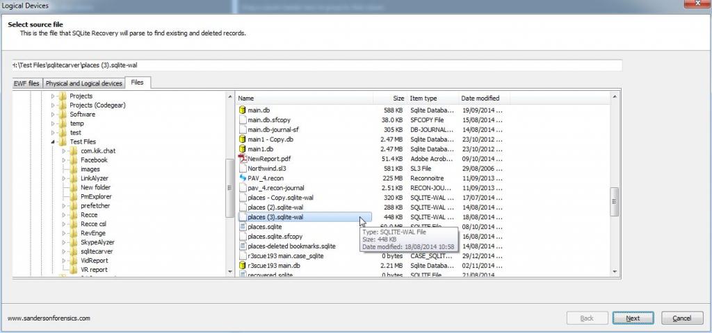
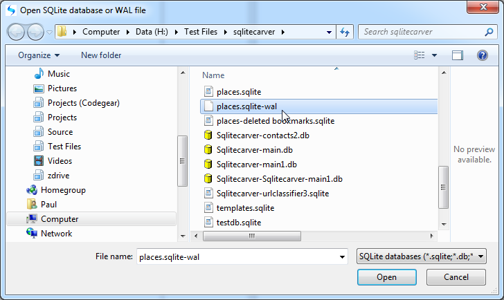
1. Select “Explore database/WAL file” from the main menu and choose a WAL file
3. Start your investigation.
The first page the investigator will see is the 32 byte WAL file header. The information of most value to an investigator here is the Page size and the WAL salt. Every additional page in the WAL is will be page size (in this case 32K) plus 24 bytes in length (the 24 bytes are referred to as WAL frame headers), the salt values from the WAL file header are repeated in every frame header.


Each record is displayed in decoded form in the records display (shown above) and selecting the start of the payload in the hex display pops up a dialogue showing the record inserted into its matching table (obtained from the schema from the associated database) and the record can now be written to a copy database for further examination using additional software such as SkypeAlyzer.
Without going into the pros and cons of this, from a forensic point of view it is irrelevant anyway, the move has had the effect of introducing a new set of artefacts and in particular a new location for stored/cached image files (pictures).
More information here: https://support.skype.com/en/faq/FA1…t-is-the-cloud
This article deals with the SQLite tables that reference to these pictures, the locations of the pictures themselves and how to join the relevant tables, decode the data held in certain blob fields and create a report showing who sent what to whom including the pictorial evidence where possible.
At the end of the article, I will have shown how the different tables fit together and will provide a Browser extension that will create the necessary tables and import the cached pictures; you will be able to run a report that shows who sent an image and when. Alongside this, it will display the original image (if sent from the machine we are investigating) and will display the cached image. From the information, if the sender is the owner of the machine we are investigating, we will be able to see if the image was sent from this machine or was sent from another device and synced with this machine. In certain cases, we will be able to see the original path on a remote users machine (i.e. when someone sends an image to us) and therefore potentially glean information re the remote users operating system.
Note: This article was prepared after looking at a small test set of Skype installations on Windows 7 and 8 PCs, as such the details within may need to be revised at a later date when more information comes to light.
While this article is quite lengthy and a little technical it is important to realise that to use the Forensic Browser for SQLite (part of the Forensic Toolkit for SQLite) to examine the Skype media cache you don’t need to understand SQL, all you need to be able to do is to apply it, and this can be done in just a few short steps that will be summarised at the end.
This particular investigation started off when Jimmy Weg from Montana DCI contacted me and asked if I knew anything about the Skype media cache. He said that the files in the cache were created when a user/Skype synced between devices and he wanted to know if there was a way to determine the sender and recipient of the files.
At the end of this process you will be able to run a simple script that prompts you for the relevant file locations and that then creates the necessary queries such that you can run an installed report in the Forensic Browser for SQLite that looks as below and can be exported directly as a HTML report. No knowledge of SQL is required by the user.

C:\Users\Paul\AppData\Roaming\Skype\r3scue193\medi a_messaging\media_cache
The content, as can be seen below, were cached image files with some odd naming conventions and associated files that looked from their names like they might be thumbnail images.


A root around in the asyncdb subfolder of media_cache shows a cache_db.db file that on examination is unsurprisingly an SQLite database. This database contains just one table “assets” the content of which is shown below in the Forensic Browser for SQLite.
The access_time field records the 100 nanosecond intervals since 1/1/970 and the Forensic Browser for SQLite can decode this (and apply a timezone offset should I desire) for me. The serialized_data field is a Binary Large OBject (BLOB) and contains what appears to be the file name from the cache (more on this later), blobs are displayed as hex by default in the Browser.

The Forensic Browser allows me to add additional databases (attach them) to the query designer and then perform cross-database queries, so I attached main.db to the Browser and started looking through the tables.
One of these tables jumped straight out at me, not least because I recognized the name of my bike (a Capra) and the picture I had taken at the Falmouth Tall Ships event last year, pictures of both appear above.

We still need to show who the sender and receiver are, so back to the tables in main.db. I know that Skype often stores system status information in the messages table so the first thing I did was to look in the messages table at the approximate times recorded in the table above, this came up trumps. There were a number of records that were related to my previous query, these records all had a type ‘201’, so I was able to quickly build a visual query on just type 201 records from the messages table. You can see the rows in the original_name column above appear in the screenshot below embedded in the body_xml column:


You can find more information on the SQLite core functions here:
https://www.sqlite.org/lang_corefunc.html
We can now join the messages table to the MediaDocuments table and The MediaDocuments table to the assets table. The only thing that remains to be done is to import the original images if they exist from the original folders (original_name) and the cached images from the media_cache folder. While this can be done using the built-in functionality of the Forensic Browser as I am providing a Browser extension to create the joins on the different tables and extract the cached filenames from the serialized_data column it makes sense for me to also import the pictures in the extension. This means that you just need to run a single program and follow a few prompts to create your report. So all that needs to be done by you is to run the extension (if you are a Forensic Browser user and haven’t got a copy of this browser extension then please get in touch).

Select run and choose the case file

This next step is optional and you can just hit cancel.
Choose the path to the root of your extracted data and choose an offset to ensure valid paths. In the dialogue below the first three “file names to find” are possible valid files from the local file system, we are investigating. When the file path (from character 3) is appended to the prefix then a valid path on the investigation machine is obtained – then the extension checks the file path for any existing matching files and shows them in the bottom memo. At this point (when valid file paths show in the bottom memo) you can select OK to continue.

When the Browser extension completes, hit “Close”, there will be two new SQL queries saved in the Query Manager as below:

The first query “Full Query” returns every row from the combined tables (as well as any pictures that were imported). The second query “Abbreviated Query” returns a subset of the main columns from the query. You are of course encouraged to modify these queries to get the report you would like.
The remaining three queries are the SQL for the VIEWS used by the two main report generating queries above. While a single compound query could be written it is a useful practice to break down complex queries in to smaller subqueries/views in order to simplify the problem.
An example of the output of the abbreviated query is shown below:
There are some excerpts from the results shown below that help explain what we are seeing. The main.db file and the extracted profile image are all from my office Windows 7 PC.
First off, note there are two rows for each sent picture, this is because the media_cache folder holds two pictures. One full size and one thumbnail for each transfer.
The first two rows show a picture that was sent by a colleague in Canada to me, the orginal_name column contains the name of the picture on his device. The author and from_dispname columns contain his skype user name and “friendly” name. The dialog_partner column is also populated with his name.
The second two rows show a picture that I sent to him from my Surface Pro PC. Note that the dialog_partner column is not populated but my colleagues name does appear in the chatname column. The original_name column contains the file name on the surface pro. My user name is correctly shown in the author and from_dispname columns.
Rows 5 and 6 show a file that was sent from my iPhone to a second Skype test account I have that was running on a different machine (another laptop). Note the original_name column is empty, this may be because one or both devices does not support the new photo sharing functionality at this time.
Finally in this screenshot the bottom two rows show a picture sent from this PC (Windows 7 desktop) to another colleague Gary, in this case the original_name field contains the fully qualified path of the original picture on the Windows 7 PC, however the last two columns (original_filename and original_image) are not populated because the original picture has since been deleted – although helpfully Skype has maintained a cached copy for us.


For instance, I replace the following query with the view name “Messages201”
SELECT Messages.”timestamp”,
Messages.chatname,
Messages.author,
Messages.from_dispname,
Messages.dialog_partner
FROM Messages
WHERE Messages.type = 201
I can then use either the full query or just “SELECT * FROM messages201” to get the same results. The three VIEWS I create are available for use by the Forensic Browser user as follows:


The row in the messages201 view has an ID of 5743 (all records in the Skype main.db have a unique ID irrespective of what table they reside in), the record in MediaDocuments has an ID of 5742, i.e. one previous. The edited_timestamp in Messages201 is 2015/03/05 20:20:03 and the access_time in assets is 2015/03/06 20:20:04.
If any Forensic Browser users need help with any of the SQL referred to above or installed into the Query Manager by the browser extension (or indeed any SQL query at all) then please get in touch and I’ll do what I can to help.
I had reason recently to look at Skype ChatSync files to recover the IP addresses held within and I needed to get these into a report. For those of you that aren’t aware when Skype is syncing data between two different accounts, it uses ChatSync files to transfer this data. The data held within is, for the most part, duplicated in the main.db file (after all that is what the sync part of ChatSync refers to). However, and most interestingly for forensic purposes, usernames and IP addresses are also stored within these files.
I have therefore written a Forensic Browser for SQLite extension that parses the folder containing these files and for every file records the following information in a new SQLite database:
It struck me when writing this application that I could also obtain some location information from an online service and display this information within a Skype report and further I could use the built-in mapping functions of the Forensic Browser for SQLite to display maps related to the latitude and longitude fields obtained from my IP lookup service.
Of course, location information based on IP addresses needs to be carefully considered as IP addresses will often be the of a service provider. Nevertheless on examination of the IP addresses and particularly associated maps for my own Skype username quickly revealed some interesting locations.
The screenshot below shows the output of this process with three maps at different scales shown alongside the details from the ChatSync files.
The rest of the article will show how easy it is to create these reports yourself.

So, first, visit IPInfoDb and create a free account at this page http://www.ipinfodb.com/register.php you need to provide an IP address of the “server used to connect to the API gateway” I used the IP address of my router (also conveniently displayed on the page above) and all seems to work OK. You need to acknowledge an email in the normal fashion and then to wait 10 minutes after the acknowledgement before you can use the service. When the service is created you will be provided with a long alphanumeric key – you will need this later.


Select “Create geolocated images” from the “Tools” menu

The zoom levels specific the scale for each of the three created maps (0 disables a map) with 16 being the maximum “zoom in” level (i.e. street level) and 1 the minimum.
Press OK and the table will be created, this may take a few minutes as the maps are created and downloaded via the open street map server.


